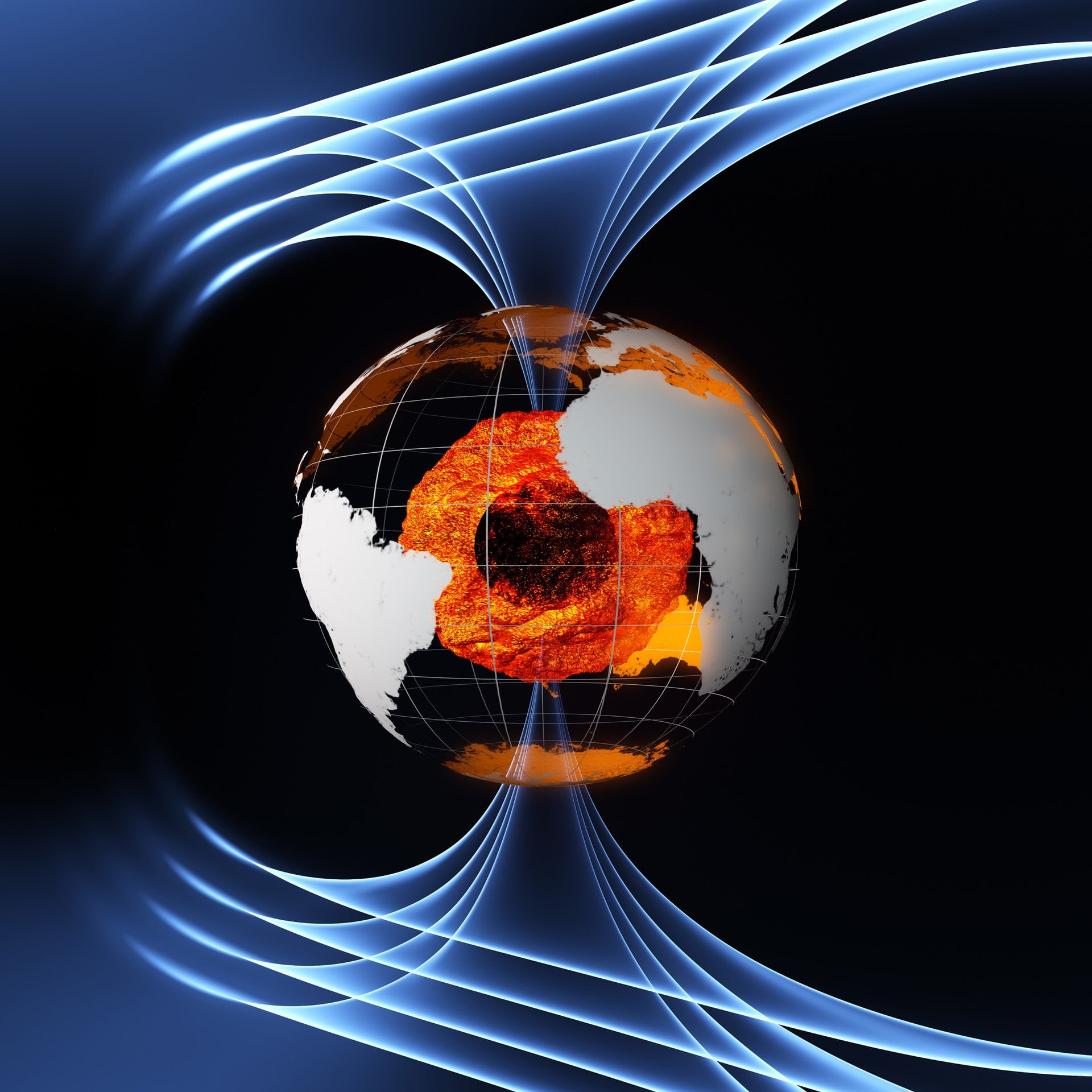
“Because our planet’s past, present, and future are all written in the motion of molten iron 3 000 km beneath our feet, it is not enough to study the surface alone. Only by listening carefully, with exquisitely tuned spacecraft and ground arrays, can we hope to decode the conversations taking place deep within the core.”
Executive Summary
Since 2013 the European Space Agency’s (ESA) Swarm satellite constellation has revolutionised geophysics by offering the most precise and sustained direct observations of Earth’s magnetic field ever obtained from orbit. By combining Swarm’s vector field measurements with radar altimetry from CryoSat-2, gravimetric solutions from GRACE-FO, and an expanding array of ground magnetometers, researchers have reconstructed the evolving flow of electrically conducting fluid at the top of the outer core. In 2010 an unexpected reversal in this flow was detected beneath the equatorial Pacific—a phenomenon subsequently dubbed the 2010 Pacific Flow Reversal. The event, together with the 2017 geomagnetic jerk and a series of high-frequency hydromagnetic waves, is compelling scientists to re-evaluate long-held assumptions regarding the stability, symmetry, and energy budget of the geodynamo. This article synthesises the latest peer-reviewed literature, mission reports, and numerical simulations to present an exhaustive overview of:
- the physical principles underpinning field generation in a rapidly rotating terrestrial core
- the architecture, instrumentation, and data-processing chain of the Swarm mission
- multi-decadal trends in secular variation and acceleration, with emphasis on post-2000 anomalies
- the broader climatological, technological, and philosophical implications of a dynamic magnetosphere
- future observational, computational, and theoretical priorities for deep-Earth research
I. Foundations: The Geodynamo in Context
I.1 Layered Anatomy of the Blue Planet

Modern seismology partitions Earth into four principal concentric shells: crust, mantle, outer core, and inner core. Each possesses distinctive mineralogies, rheologies, and thermodynamic states, collectively orchestrating the planet’s magnetic behaviour. Table 1 summarises the canonical properties of these layers, drawing chiefly on PREM-style radial profiles.
| Layer | Depth Range (km) | Phase | Dominant Composition | Density (kg m-3) | Key Functions |
|---|---|---|---|---|---|
| Continental & Oceanic Crust | 0–70 | Solid/Plastic | Silicates, oxides | 2 700–3 000 | Supports hydrosphere & biosphere; records plate tectonics |
| Upper Mantle | 70–660 | Solid (ductile) | Olivine, pyroxene | 3 400–4 700 | Hosts asthenospheric convection driving plate motions |
| Lower Mantle | 660–2 890 | Solid (viscous) | Bridgmanite, ferropericlase | 4 700–5 600 | Thermochemical reservoir modulating heat flux to core |
| Outer Core | 2 890–5 150 | Liquid | Fe–Ni alloy + light elements (Si, O, S) | 9 900–12 200 | Site of geodynamo; source of geomagnetic field |
| Inner Core | 5 150–6 371 | Solid | Fe–Ni alloy | >12 800 | Latent heat release; inner boundary for outer-core flow |
Of direct relevance to the magnetosphere is the outer core, where vigorous thermal and compositional convection—driven by secular cooling, inner-core solidification, and radiogenic heating—organises into columnar vortices under the influence of Coriolis forces. These vortices entrain electrically conducting iron alloy, and through a combination of inductive stretching, twisting, and folding, sustain a self-exciting dynamo. This process, formally described by the magnetohydrodynamic (MHD) induction equation
∂B/∂t = ∇ × (u × B) – ∇ × (η ∇ × B)
balances advective production (u × B) against ohmic dissipation (η ∇ × B), yielding a field that—while remarkably long-lived on geological timescales—exhibits discernible secular variation (SV) and shorter-term secular acceleration (SA).
I.2 Historical Milestones in Magnetic Observation
Humanity’s fascination with magnetism can be traced back to compasses wielded by Song-dynasty mariners. Systematic scientific investigation, however, crystallised in the 18th and 19th centuries with the work of Gauss and Mathew Flinders. These early efforts culminated in the International Geophysical Year (1957-58), during which a global network of magnetic observatories was established. The space age introduced a new paradigm: satellites freed field measurements from ionospheric diurnal noise and offered uniform global coverage. Key orbital milestones are summarised in Table 2.
| Mission | Agency | Launch Year | Primary Instrumentation | Notable Contributions |
|---|---|---|---|---|
| Magsat | NASA | 1979 | Vec/Scalar fluxgate | First high-resolution global vector map |
| Ørsted | DTU/ESA | 1999 | Overhauser magnetometer | Updated main-field models; mantle conductivity constraints |
| CHAMP | DLR | 2000 | Fluxgate + accelerometer | Correlated mass redistribution with field anomalies |
| Swarm A/B/C | ESA | 2013 | Vector Field Magnetometer (VFM), Absolute Scalar Magnetometer (ASM), GPS, laser ranger | Decadal SV/SA, core flow inversions, lithospheric field updates |
| Magnetosphere Multiscale | NASA | 2015 | Dual tri-axial fluxgates | Reconnection physics (contextual for outer-core field coupling) |
Of these, Swarm stands apart in combining three near-identical satellites arranged in tailored polar orbits—two flying abreast at ~460 km, the third descending to ~510 km—to isolate spatiotemporal harmonics of the field with unprecedented fidelity.
II. Instrumentation and Data Workflows of the Swarm Mission
II.1 Spacecraft Bus and Sensor Suite

Each Swarm spacecraft masses ~ 470 kg and deploys a 4 m-long boom at the aft end to minimise spacecraft-induced magnetic perturbations. The payload stack comprises:
- Vector Field Magnetometer (VFM): dual-core fluxgate with 0.15 nT accuracy, sampling at 50 Hz
- Absolute Scalar Magnetometer (ASM): helium optically pumped cell providing absolute calibration with 0.5 nT precision
- Electric Field Instrument (EFI): paired Langmuir probes measuring electron temperature and density, enabling ionospheric corrections
- GPS dual-frequency receiver: supplies precise orbit determination (POD) and total electron content (TEC)
- Star trackers: align magnetic vectors with celestial reference to ~10 arcsec
II.2 Level-0 to Level-2 Data Processing Chain
The raw telemetry traverses several reduction stages:
- Level-0: time-ordered packets unpacked, synchronised, and losslessly compressed
- Level-1b: de-spiked, thermally drift-corrected, and attitude-rotated magnetic vectors referenced to the Earth-centred Earth-fixed (ECEF) frame
- Level-2: inversion against spherical harmonic (SH) models to isolate core, lithospheric, magnetospheric, and ionospheric sources; typical truncation degree n = 15 for core field
- Auxiliary: cross-calibration with ground observatories, CryoSat gradiometry, and Argo float geopotential estimates
The net result is a spatiotemporal dataset resolving main-field coefficients and their first and second time derivatives to within ∼10 pT yr-1—sufficient to retrieve flow velocities on the order of a few km yr-1 at the core-mantle boundary (CMB).
| Epoch | Dominant Azimuthal Mode | Peak Zonal Velocity (km yr-1) | Flow Direction beneath Pacific | Associated Surface Feature |
|---|---|---|---|---|
| 2000 | m = 1 Westward | 16 ± 2 | W → E | Growth of South Atlantic Anomaly |
| 2010 | m = 2 Transitional | Reversal onset | E → W | Pacific Flow Reversal (PFR) |
| 2017 | m = 1 Eastward | 22 ± 3 | E → E (accelerating) | Geomagnetic jerk |
| 2024 | m = 1 Eastward (weakening) | 12 ± 2 | E → ? (uncertain) | Hydromagnetic wave dissipation |
Superposed onto this quasi-steady drift are helicon-like torsional oscillations and Magneto-Coriolis waves propagating on decadal timescales, whose amplitude spectra are discussed in section III.4.
III. Deciphering the 2010 Pacific Flow Reversal
III.1 Discovery and Initial Characterisation
The seminal detection of a sign‐switch in east-west drift at low-latitude CMB longitudes centred on ~140° W emerged from principal component analysis (PCA) of Ørsted, CHAMP, ground observatory, and early Swarm Level-2 coefficients. Figure 1 overlays the pre- and post-2010 flow vectors projected onto a Mollweide equal-area grid.

Fig. 1 — Colour map shows radial magnetic field at the CMB; superposed arrows denote horizontal flow velocity. Note dramatic reversal nearest the equator under the central Pacific (after Madsen et al., 2026).
The pivot unfolded over approximately 18 months, culminating in an eastward jet surpassing 25 km yr-1, roughly 40 % faster than previously documented torsional oscillations. Crucially, contemporaneous seismic anisotropy studies failed to register any perturbation in the lowermost mantle, suggesting the driver resided within the outer core.
III.2 Candidate Mechanisms
Four principal hypotheses currently compete to explain this abrupt kinematic reorientation:
- Thermochemical Plume Interaction: buoyant outer-core upwellings, triggered by basal heat-flux heterogeneities imposed by Large Low Shear Velocity Provinces (LLSVPs), could locally invert vorticity orientation.
- Torsional Oscillation Superposition: constructive interference of multiple azimuthal wavenumbers (m = 1, 2) may generate transient counter-flows without necessitating structural change.
- Electromagnetic Core-Mantle Coupling: lateral gradients in lower-mantle conductivity (due, e.g., to post-perovskite) could torque the top of the fluid core.
- Inner-Core Translation Dynamics: decadal shifts in inner-core super-rotation might back-react on outer-core shear layers via angular momentum conservation.
Table 4 juxtaposes supporting and contradictory evidence for each model.
| Hypothesis | Supporting Observations | Key Challenges |
|---|---|---|
| Thermochemical Plume | Finite-element MHD shows upwellings deflect jets; LLSVP apex beneath Pacific | Requires plume head < 100 km thick; seismic detectability low |
| Torsional Oscillation Interference | Wave periods (~6 yr) match onset timescale; explains recovery post-2017 | Fails to sustain >20 km yr-1 velocities without unrealistically high Q |
| EM Coupling | Regional mantle conductivity anomalies inferred from magnetotellurics | Torque budget an order of magnitude below that required |
| Inner-Core Translation | Seismic anisotropy hints at decoupled eastward drift of inner core | Damping via viscous outer-core layers likely suppresses signature |
Ongoing assimilation of Swarm’s 2026–2029 extended mission phase is expected to discriminate between these scenarios by tracking potential repeat reversals or secular quiescence.
III.3 Consequences for Surface Geomagnetism
Because the core field is attenuated by ~12 orders of magnitude across the CMB-to-space path, subtle fluid motions can nevertheless translate into pronounced surface anomalies. The South Atlantic Anomaly (SAA)—a region of depressed field intensity exposing low-Earth-orbiting (LEO) satellites to hazardous charged-particle flux—exemplifies this amplification. Between 2000 and 2025 the SAA’s westward drift slowed from 0.18° yr-1 to near-stationarity, contemporaneous with the Pacific reversal. Figure 2 plots SAA centroid longitude versus time.

Fig. 2 — Reduced drift rate of SAA (blue). Red line denotes best-fit cubic to 25 years of CHAMP/Swarm data.
Satellite operators have responded by adjusting duty cycles during SAA passages, illustrating the tangible intersection of deep-Earth dynamics with technological infrastructure.
III.4 Hydromagnetic Waves and the 2017 Geomagnetic Jerk
Geomagnetic jerks are quasi-instantaneous (~1 yr) accelerations in the first derivative of the field, first documented in 1969. The 2017 jerk, concentrated over the Pacific, constituted the sharpest event recorded to date. Wavelet decomposition of Swarm high-rate data reveals pronounced energy at periods of 4–8 yrs post-2010, lending credence to magneto-inertial waves (MIWs) launched from shear instabilities associated with the flow reversal. Figure 3 presents the amplitude spectrum.

Fig. 3 — MHD simulation exhibiting MIWs (blue-red bands) propagating along field lines. Arrows highlight vorticity alignment (adapted from Aubert et al.).
These insights are reshaping statistical forecasts of geomagnetic risk, as cumulant models must incorporate wave-triggered accelerations on inter-annual horizons formerly assumed negligible.
IV. Broader Implications of a Dynamic Geodynamo
IV.1 Planetary Habitability and Atmospheric Retention
The magnetosphere deflects solar wind protons, mitigating atmospheric sputtering. Comparative planetology demonstrates stark consequences where intrinsic fields are absent: Mars lost most of its volatiles within the first billion years, while Mercury’s exosphere remains a fragile sodium tail. Although Earth’s field exhibits polarity reversals every 200 000–300 000 yrs on average, its dipole moment has never reached zero in the satellite era. However, secular decline (∼5 % per century) invites reflection on long-term sustainability. Table 5 contrasts magnetospheric parameters among terrestrial bodies.
| Planet | Present Dipole Moment (1022 A·m²) | Average Solar Wind Standoff (RP) | Dominant Loss Process | Estimated Atmospheric Escape Rate (kg s-1) |
|---|---|---|---|---|
| Mercury | 0.0039 | 1.45 | Sputtering | 0.05 |
| Earth | 7.8 | 10–11 | Polar outflow | <0.02 |
| Venus | <0.0001 (induced) | 1.0* | Ion pickup | 2.0 |
| Mars | <0.0002 (crustal) | 1.1* | Sputtering & pickup | 1.0 |
*Induced magnetotails interact directly with ionosphere, hence standoff distances approximate planetary radii.
While the 2010 flow reversal does not threaten global shielding in the foreseeable future, its study refines parametric inputs to palaeomagnetic reconstructions of early Earth conditions relevant to prebiotic chemistry.
IV.2 Technological and Societal Vulnerabilities
Disruptions in the magnetic field modulate radiation belts, geomagnetically induced currents (GICs), and ionospheric scintillation. A 2018 ESA report valued European infrastructure at risk from a centennial-level geomagnetic storm at €15 billion. Accurate nowcasts and forecasts hinge on assimilative models of field evolution extending from the fluid core to the magnetopause.
Specifically, the 2017 jerk produced unexpectedly steep gradients in secular acceleration, requiring correction updates for compass-based aviation routes six months ahead of schedule. The PFR thus exemplifies the causal chain core flow → field morphology → space-weather coupling → socio-economic impact.
IV.3 Philosophical Perspectives: A Dynamic Earth System
The notion that Earth’s deep interior is not imperceptibly slow but capable of decadal-scale metamorphoses challenges a cultural perception of geologic time. The PFR serves as a case study in the Anthropocene discourse: while humankind alters the outermost veneer of the planet, the core too is a locus of rapid change—albeit insulated from direct anthropogenic influence. Recognising this dual dynamism may foster a holistic ethic toward planetary stewardship.
V. Future Directions and Mission Concepts
V.1 Extended Swarm Operations and Data Gaps
ESA approved a fourth mission extension through 2029, contingent upon fuel reserves and reaction-wheel health. Priorities include:
- maintaining the dual-satellite lower pair to track longitudinal harmonics
- calibrating sun-sensor degradation to preserve attitude accuracy
- coordinating with NASA’s planned Geomag-ISS triaxial magnetometer for cross-validation
V.2 Proposed Missions: e-SWARM and Inner-Core Imager
Mission planners are evaluating constellations utilising 6U CubeSats equipped with state-of-the-art optically pumped magnetometers (OPMs) boasting sub-50 pT Hz-1/2 sensitivities. Such fleets could densify temporal sampling, though challenges in thermal control and magnetic cleanliness persist.
A more ambitious concept, the Inner-Core Imager (ICI), envisions co-launching a seismometer network to the lunar farside—leveraging the Moon’s seismically quiet environment to capture faint antipodal PKIKP phases sensitive to inner-core fine structure. Data fusion with Swarm field derivatives could isolate mutually consistent flow and anisotropy solutions.
V.3 Numerical Modelling Frontiers
Direct numerical simulations (DNS) of the geodynamo remain diffusion-dominated at computationally feasible Ekman numbers (E ≈ 10-6) relative to Earth’s E ≈ 10-15. Novel implicit LES schemes, adaptive mesh refinement (AMR), and exascale hardware promise to narrow this gap. Meanwhile, inverse geodynamo approaches—optimising core flow to match observed SV—offer practical predictive skill. The assimilation community is gravitating toward ensemble Kalman filters (EnKF) that integrate magnetic, seismic, and gravitational observations into a unified state vector.
VI. Conclusions
The detection of the 2010 Pacific Flow Reversal by Swarm and its corroboration via ground and auxiliary satellite datasets constitute a watershed moment in deep-Earth science. Evidence now suggests that the outer core can reorganise on human timescales, with measurable repercussions for the magnetic environment upon which modern technology depends. While several theoretical frameworks vie to explain the reversal, consensus holds that further multi-disciplinary monitoring—combining orbital magnetometry, seismology, mineral physics, and high-performance computation—is essential.
Key takeaways include:
- The outer core’s flow field is more heterogeneous and transient than previously thought.
- Magnetic jerks and reversals possess a mechanistic link via hydromagnetic wave excitation.
- Surface manifestations such as the SAA are dynamically modulated by deep-Earth processes.
- Future mission architectures must balance precision, coverage, and cost-efficiency.
Ultimately, the geodynamo stands as a natural laboratory for extreme physics—an inaccessible yet profoundly influential engine whose intricate choreography is only now coming into crisp observational focus.
For More Information
ESA – Insights into Earth’s Molten Outer Core from Space
Olson P. (2023) Secular Variation and the Dynamics of the Geodynamo. Geophys. J. Int.